Frequency difference of arrival (FDOA) — also called differential Doppler — is a passive geolocation technique that determines an RF emitter's position from the difference between the Doppler shifts the same emission produces at two receivers that are moving relative to it. The measured difference is typically a few hertz down to millihertz, and it constrains the emitter to an iso-Doppler curve; intersected with the TDOA hyperbola from the same receiver pair, it produces a fix without transmitting anything toward the target. It is the standard second observable wherever collectors move: aircraft, UAVs and satellites.
The Doppler physics behind FDOA
A receiver that moves toward or away from an emitter measures a shifted carrier: the shift is the line-of-sight closing velocity divided by the wavelength. Two receivers with different lines of sight measure different shifts even when the emitter's own frequency is unknown and unmodulated. In the standard narrowband model (relative velocities are tiny compared with c, so the received signal is a delayed, frequency-shifted replica of the transmitted one):
Doppler at receiver i:   d_i = v_los,i / lambda                     [Hz]
FDOA (receiver B - A):  f_FDOA = d_B - d_A
                              = (1/lambda) * ( v_B . u_B  -  v_A . u_A )

u_i = unit vector from receiver i toward the emitter
v_i = velocity vector of receiver i,  lambda = c / f0
The unknown transmit frequency cancels in the difference — you never need to know the emitter's exact carrier — but both receivers must share a frequency reference stable to a small fraction of the FDOA you intend to measure. The scale of the numbers: at 300 MHz (wavelength about 1 m), a UAV flying 50 m/s sees at most ±50 Hz of Doppler; at 12 GHz, every 1 m/s of line-of-sight motion is 40 Hz. Resolving the difference between two such shifts to millihertz precision drives most of the system design on this page.
Iso-Doppler contours: the geometry of an FDOA measurement
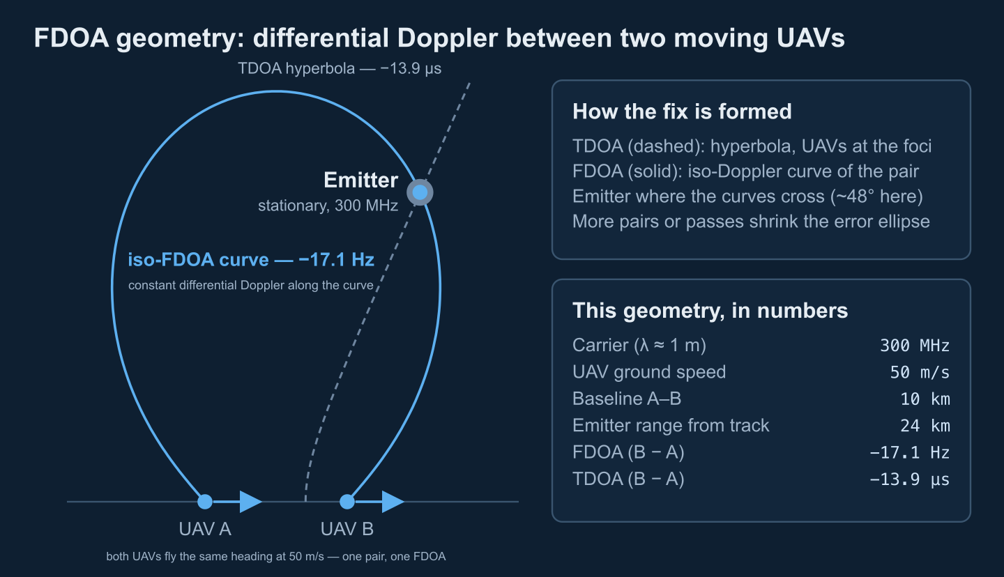
Each measured FDOA value defines a locus: the set of emitter positions producing exactly that differential Doppler for the known receiver positions and velocities. These iso-Doppler (iso-FDOA) contours are the counterpart of TDOA's hyperbolas, but they are not conics. A recent algebraic-geometry analysis shows the two-sensor FDOA equations form a degree-eight polynomial system (Duflot, Cheney and Given, 2024), and Pine, Pine and Cheney (IEEE TAES, 2021) catalogue how the curves behave:
- Near field (emitter range comparable to the baseline): the contours bend around each sensor with horn-like singularities at the sensor positions — no tidy closed-form treatment as TDOA enjoys.
- Far field, unequal sensor velocities: the contours straighten into lines through the sensor formation, so FDOA carries direction-only information — the same information TDOA already provides, which explains the poor far-field performance of some unequal-velocity TDOA/FDOA solutions.
- Far field, equal velocities (an in-trail pair): the direction-only leading term cancels, genuine range information survives, and the iso-Doppler curve keeps crossing the TDOA hyperbola transversally out to long range. This is one reason two aircraft or UAVs flying the same heading is such a productive geometry.
Sensitivity decays with range: move the emitter twice as far away and the same position change produces roughly a quarter of the FDOA change (about v * b / (lambda * R^2) at broadside for an in-trail pair with baseline b). Position from FDOA is thus progressively ill-conditioned with range — satellite systems compensate with 40× shorter wavelengths and velocities measured in km/s.
Why at least one collector must move
No relative motion, no FDOA. With a stationary emitter and two stationary receivers, both Doppler shifts are zero and the measurement is identically uninformative — a static ground network must rely on TDOA or angle of arrival alone. Three regimes matter in practice:
- Stationary emitter, moving receivers — the canonical airborne case. Any motion that makes the two line-of-sight velocities differ produces FDOA: different headings, or simply different positions along one flight path (an in-trail pair sees different bearing angles to the emitter, hence different Dopplers, even at identical speed and heading).
- Moving emitter, stationary receivers — FDOA is again measurable, now as the difference of the emitter's Doppler at the two sites. But the emitter's velocity vector enters the equations as additional unknowns, so the solver must estimate position and velocity jointly and needs correspondingly more measurements.
- Unmodeled emitter motion is a bias, not noise — in the worked example below, an emitter creeping 10 m/s along the baseline while you assume it is stationary shifts FDOA by 3.4 Hz — 3.7 km of apparent displacement that averaging more dwells cannot remove.
Where does the motion come from? UAVs and aircraft fly fast but must log their own velocity accurately; low-Earth-orbit satellites sweep tens of kilohertz of Doppler past the emitter during a pass; and even nominally geostationary relays move by metres per second — enough that satellite interference geolocation must correct for Doppler that drifts during the collection.
TDOA vs FDOA vs AOA: which technique when
TDOA and FDOA are estimated in the same operation (next section) and solve for the same emitter, but they fail in different places, and AOA remains the third pillar. The table summarizes the trade space; our overview of RF geolocation in defense develops each technique at introductory depth.
| TDOA | FDOA | AOA | |
|---|---|---|---|
| Measures | Difference in arrival time (path-length difference) | Difference in Doppler shift (line-of-sight velocity difference) | Bearing from a calibrated antenna array |
| Position locus | Hyperbola with the sensor pair as foci | Iso-Doppler curve — not a conic; set by both velocity vectors | Bearing ray; fix by triangulation |
| Hard prerequisite | Nanosecond-class time synchronization | Relative motion + millihertz-class shared frequency reference + known platform navigation | Array calibration and aperture |
| Excels at | Wideband signals, long baselines, static ground nets | Narrowband signals, long coherent dwells, fast platforms | Short range, fast first bearing, single-platform cueing |
| Fails at | Narrowband carriers (no timing sharpness), collinear geometry | Static pairs, far-field equal-heading degeneracy, drifting references, unmodeled emitter motion | Long range (error grows linearly), multipath, small apertures |
| Typical collectors | Ground sensor networks, UAV swarms | Aircraft, UAV pairs, LEO and GEO satellites | Ground DF rings, mobile single platforms |
The complementarity is the operational point: TDOA precision scales with signal bandwidth, FDOA with coherent integration time — a narrowband carrier that starves TDOA can still yield millihertz FDOA. Fusion and the error-ellipse arithmetic to weight it are covered in our geolocation accuracy and CEP guide, the sensor-topology view in direction finding network architecture.
Joint TDOA/FDOA estimation: the cross-ambiguity function
TDOA and FDOA are not measured separately: the pair's complex baseband signals are correlated across a two-dimensional grid of candidate delays and frequency offsets — the cross-ambiguity function (CAF), introduced for this problem by Stein's 1981 ambiguity-function work and still the standard formulation:
CAF(tau, nu) = integral over t in [0, T] of
               s1(t) * conj( s2(t + tau) ) * exp( -j * 2 * pi * nu * t ) dt

peak of |CAF(tau, nu)|   ->   ( TDOA, FDOA ) estimate for the pair
Along the delay axis the peak is about 1/B wide (B = signal bandwidth); along the Doppler axis about 1/T wide (T = coherent integration time). Those are resolution widths, not accuracy limits — interpolating around the peak recovers a fraction of a bin — but they set the search grid. Practical engines follow the pattern Stein established: form the lag product s1(n) * conj(s2(n+m)) for each candidate delay m, low-pass and decimate it (the Doppler band of interest is a tiny fraction of the sample rate), and take one FFT per delay column:
# coarse CAF on a delay x Doppler grid, then refine
for m in candidate_lags:                        # delay hypothesis
    lag = s1[n0:n0+N] * np.conj(s2[n0+m:n0+m+N])  # lag product
    lag = decimate(lowpass(lag, doppler_bw), M)
    A[:, m] = np.fft.fft(lag, n=n_fft)          # Doppler slice, one FFT per lag
# quadratic interpolation of |A| around the peak -> (tdoa, fdoa)
Two refinements matter in production. First, a coarse-to-fine search: a wide grid at low resolution to find the peak, then local refinement — brute force over the full uncertainty space is computationally ruinous. Second, a Doppler-rate term: when the differential Doppler drifts during the dwell (satellite relays are the classic case), the correlation must compensate a frequency changing approximately linearly with time — the approach patented for two-satellite interference location by QinetiQ (Griffin et al., US 6,618,009), building on Haworth's earlier DTO/DFO satellite location method. Peak height and curvature also yield the covariance the solver needs to weight the pair. The CAF is the heaviest computation in the chain — one FFT per delay column, per pair, per dwell — and sits naturally on the same GPU pipeline as channelization and classification, as described in our SDR signal processing pipeline architecture.
What sets FDOA accuracy
The classical reference is the Cramér-Rao lower bound stated by Stein in 1981 (without derivation there; the signal-model fine print was later examined by Fowler and Hu, and by Yeredor and Angel). For two receivers observing the same unknown signal in additive white Gaussian noise, under the narrowband approximation:
sigma_FDOA  >=  1 / ( 2*pi * T_rms * sqrt(B * T * SNR_eff) )    [Hz]
sigma_TDOA  >=  1 / ( 2*pi * B_rms * sqrt(B * T * SNR_eff) )    [s]

1 / (2 * SNR_eff) = 1/SNR_1 + 1/SNR_2 + 1/(SNR_1 * SNR_2)

B      receiver noise bandwidth [Hz]
T      coherent collection time [s]
T_rms  rms duration of the effective window (T/sqrt(12) for rectangular)
B_rms  rms bandwidth of the signal spectrum
Read the scaling, not the constants: FDOA precision is set by integration time — doubling the coherent dwell improves sigma_FDOA by 2*sqrt(2) ≈ 2.8× — while TDOA precision is set by rms bandwidth. A 25 kHz communication signal is hopeless for sharp TDOA but excellent for FDOA given seconds of coherence. Around the bound, four engineering terms dominate:
- Reference stability. Any fractional frequency offset between the two receivers' local oscillators lands directly in FDOA. A residual 1×10⁻¹⁰ offset between two disciplined references is 30 mHz at 300 MHz — ten times the pure measurement floor in the worked example below, and far worse in GNSS-denied holdover. GPS-disciplined oscillators (GPSDO) are the baseline; OCXO or rubidium references carry holdover; fiber-distributed PTP/White Rabbit removes the problem where fiber exists.
- Platform navigation. The solver converts FDOA to position using each receiver's velocity vector; an error there is indistinguishable from a Doppler error. Commodity GNSS receivers quote 0.05 m/s velocity accuracy (u-blox NEO-M8 class) — about 70 mHz of FDOA error for a pair at 300 MHz, again an order of magnitude above the measurement floor.
- Geometry. The iso-Doppler gradient falls as 1/R², and where the iso-Doppler curve crosses the TDOA hyperbola at a shallow angle, both measurements constrain nearly the same direction and the error ellipse explodes. Near-field in-trail pairs at broadside give near-perpendicular crossings; emitters on the baseline extension or the velocity axis give degenerate ones.
- Coherence limits. The dwell cannot grow indefinitely: the signal must stay phase-coherent, the emitter roughly stationary, and for wideband signals the differential delay drifts during the dwell (0.33 μs per second at a 100 m/s range-rate difference) — negligible at 25 kHz bandwidth, dominant at 10 MHz. Hoppers and burst emitters cap the window further; the mitigation is fusing many short dwells over time.
This is the layer we build: cross-ambiguity processing chains, multi-sensor TDOA/FDOA geolocation solvers with honest covariance output, and their integration into SIGINT collection and C2 pipelines. If you are specifying an airborne, UAV or ground-network geolocation capability, tell us about your platforms and signals — we will map the achievable accuracy before anyone commits to hardware.
Worked example: two UAVs fixing a 300 MHz emitter
Two UAVs fly in trail 10 km apart, both at 50 m/s on the same heading; a stationary 300 MHz emitter lies 24 km out, 65° off the baseline axis. Receiver A closes at 28.6 m/s (+28.6 Hz), B at 11.5 m/s (+11.5 Hz): FDOA −17.1 Hz. The path difference is −4.15 km, so TDOA −13.9 μs. Around the emitter, sensitivity is 0.93 Hz/km for FDOA (1 Hz ≈ 1.1 km) and 1.25 μs/km for TDOA, and the curves cross at 48° — decent, not ideal, geometry.
Assume a 25 kHz receiver noise bandwidth and 3 dB signal-to-noise ratio at each UAV, giving an effective two-receiver SNR of about 2 dB. The Stein bounds then give the pure measurement floor (before navigation and reference errors):
| Coherent dwell T | CAF Doppler bin (1/T) | sigma_FDOA (meas.) | FDOA-only position 1σ | sigma_TDOA (meas.) | TDOA-only position 1σ |
|---|---|---|---|---|---|
| 30 ms | 33 Hz | 531 mHz | 570 m | 638 ns | 511 m |
| 100 ms | 10 Hz | 87 mHz | 94 m | 349 ns | 280 m |
| 300 ms | 3.3 Hz | 17 mHz | 18 m | 202 ns | 162 m |
| 1 s | 1 Hz | 2.8 mHz | 3 m | 110 ns | 89 m |
With one second of coherence the signal itself is no longer the limit: adding 0.05 m/s GNSS velocity error per UAV (≈71 mHz) and a 1×10⁻¹⁰ residual reference offset (30 mHz) to a 2.8 mHz measurement floor gives 77 mHz total FDOA sigma, alongside 118 ns of TDOA sigma (110 ns measurement + 42 ns clock contribution). The combined fix at 24 km is roughly 70 m × 150 m one-sigma: CEP50 ≈ 130 m, CEP90 ≈ 260 m. At a 100 ms dwell, CEP50 degrades toward half a kilometre. The strongest lever at the margin is not RF hardware — it is navigation quality, reference stability and dwell length.
Building an FDOA system: from synchronized capture to C2
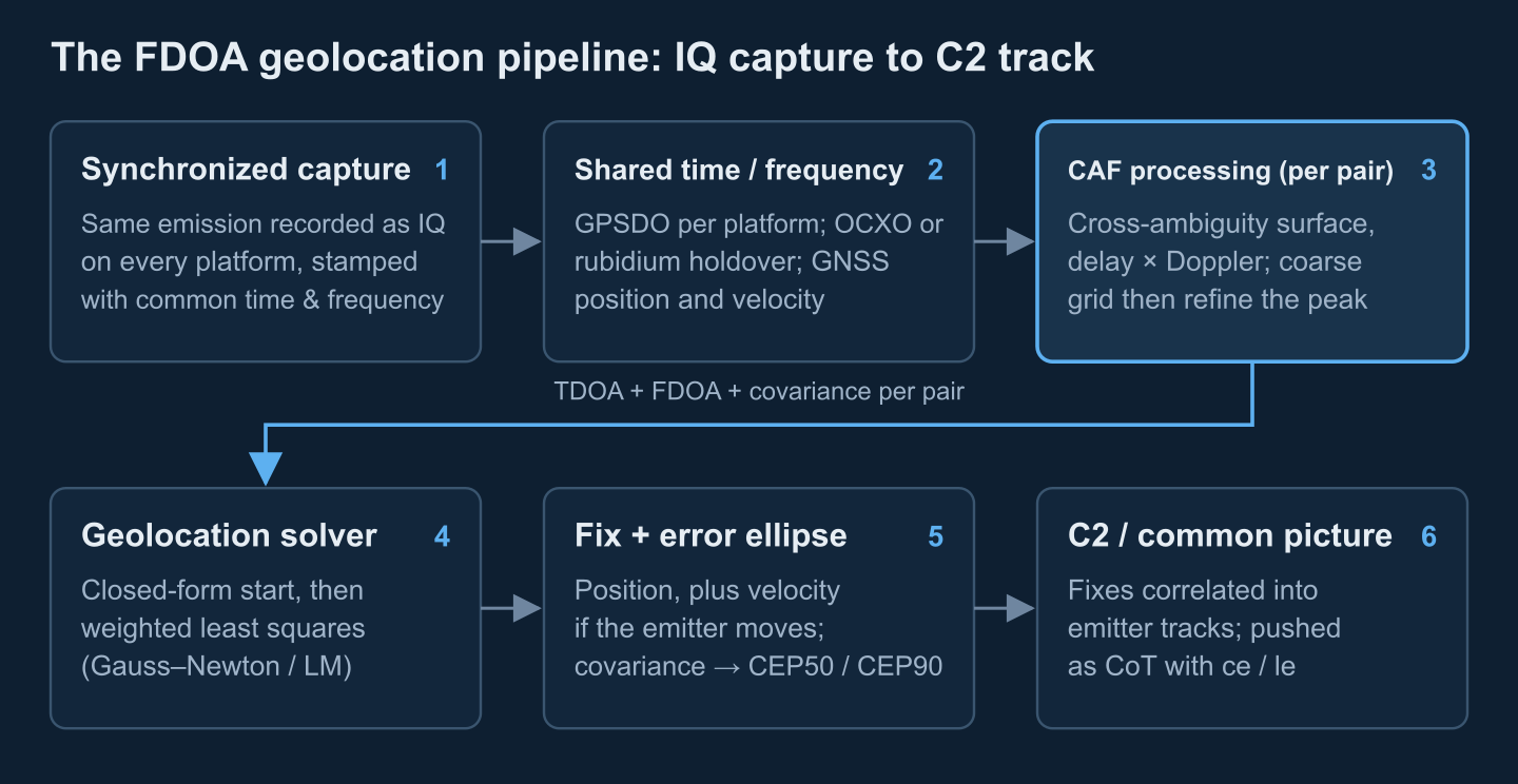
The measurement chain is only half the system; the other half keeps the platforms coherent and gets the product to a decision-maker:
- Synchronized IQ capture. Every platform records the same emission as complex baseband IQ, time- and frequency-stamped against its GPSDO. The geolocation engine is a consumer of the signal processing pipeline, not a separate radio.
- Data-link budget. Correlation needs both copies of the signal in one place: a 25 kHz channel in 16-bit IQ is about 1 Mbit/s per platform per second of dwell, a 1 MHz emission 40 Mbit/s. Ship raw IQ snippets when the link allows, process on board and ship measurements only, or centralize over fiber — the edge-versus-rear split analyzed in our SIGINT edge processing architecture.
- Calibration. Residual clock and LO offsets are estimated as nuisance parameters in the solver, ideally observed against a reference emitter at a known site. Satellite interference geolocation treats this as mandatory: known reference signals through the same two satellites remove the system offsets before the unknown emitter is solved.
- Solver. Closed-form initialization (the Ho and Chan, 1997, known-altitude solutions are the classic reference), then covariance-weighted Gauss–Newton or Levenberg–Marquardt refinement over all pairs and passes, joint emitter-velocity estimation when needed, outlier gating — and a position returned with its covariance, never a bare coordinate.
- Output to C2. Fixes correlate into tracks in the bearings database, and time-sensitive ones go to the common operating picture as Cursor on Target with
ce/leaccuracy fields set from the error ellipse — see our annotated CoT message examples. The surrounding architecture is covered in the SIGINT platform architecture guide.
Where FDOA earns its keep
Satellite interference geolocation is the flagship application: an interfering uplink captured through two adjacent geostationary satellites yields DTO/DFO (the satellite community's names for TDOA/FDOA), calibrated by reference signals, locating the interferer on the ground — its drifting differential offsets are what forced the Doppler-rate compensation described above. Airborne SIGINT treats TDOA/FDOA as the default fix mode against stationary emitters: platform motion is free and successive fixes along the flight path multiply into a tight track. UAV pairs put the worked example into practice at low cost — against drone command links, FDOA from moving collectors complements the techniques in our HackRF drone detection analysis. And wherever the narrowband emitter defeats TDOA, FDOA is the observable that still works.
When FDOA is the wrong tool
Static pairs with a static emitter measure nothing. Long-range, unequal-velocity geometries collapse into direction-only information, so a fast mover paired with a ground station can produce confident-looking fixes that are badly conditioned in range. Moving emitters bias the solution unless velocity is estimated jointly. The reference and navigation demands are unforgiving: millihertz FDOA at 300 MHz is a 10-11-class frequency measurement, and GNSS denial attacks it both directly (no discipline, no velocity) and through holdover drift. Hoppers and burst emitters cap the coherent integration the accuracy story rests on. When the signal is wideband, the sensors static and the time transfer excellent, plain TDOA is simpler and better; when the target is close and a bearing is needed in the first second, AOA wins the race. The strongest systems refuse to choose — they fuse.
Build the geolocation engine, not just the diagram
We build CAF processing chains, multi-sensor TDOA/FDOA geolocation solvers with covariance output, and their integration into SIGINT collection and C2 pipelines. Tell us about your platforms, bands and emitters.
Prepared by the Corvus Intelligence engineering team, which builds passive geolocation and SIGINT processing software for defense collection programs. About Corvus Intelligence →